
Friendly syntax ● Deterministic algorithms ● Easy workflow ● Free
| Variable | Init | Min | Max | Final Value | |
|---|---|---|---|---|---|
| 1 | A | 1 | 0.04 | 1.00 | 0.04159 |
| 2 | B | 0 | 0.00 | 0.24 | 0.03799 |
| 3 | C | 0 | 0.00 | 0.92 | 0.92042 |
We provide students, instructors, and engineers with a simple, structured workflow: define your model in plain text, run a deterministic solver, and review the results, supported by plain‑text input for reproducible collaboration and verbose reports for verification.
Explore these examples to learn the simple problem entry syntax. Each example popup shows the problem input in the left panel and the solution output in the right panel.


 Using an AI assistant?
Copy the PolymathPlus AI context.
Our support team typically replies to common requests/queries within two business days. For technical questions, enhancement requests, or bug reports, email admin@polymathplus.org with a brief description and any screenshots.
Below you'll find common support questions and answers:
PolymathPlus is math-solving software designed for students, scientists, and engineers, built to handle various numerical problems such as nonlinear equations, ordinary differential equations, linear/polynomial/nonlinear curve-fitting regression, and more.
At its core, it is a deterministic computational engine that applies well-established, rigorously validated numerical algorithms to solve mathematical and engineering models. For the same model and inputs, it produces reproducible results, which is essential for verification, traceability, and design confidence. This is fundamentally different from heuristic AI systems, which can generate variable outputs and may not always provide the consistency or numerical reliability required for engineering problem-solving.
Our goal is to deliver a user-friendly yet powerful math-solving tool that remains accessible and affordable for users around the world. With PolymathPlus, you can enter a math problem in plain text and instantly receive a numeric solution accompanied by a comprehensive report—all with a single click.
Yes. PolymathPlus offers a free, feature-rich online package.
You can try the solver immediately as a guest — no account needed. Guest users have full solver capabilities but cannot save their programs.
Consider registering for a free account to enable program storage and remove guest‑level limitations. The free package is designed for individual users. Organizations are asked to register their site (which is free) for their users.
Yes — PolymathPlus works on virtually any modern device via the web browser.


The online version works through all major browsers—including Chrome, Safari, Opera, Firefox, and Edge—on both Windows and macOS laptops and desktops. You can also access PolymathPlus on Android and iOS smartphones or tablets using the supported web browsers.
PolymathPlus is currently available only as an online service. Users who previously purchased licenses may continue using the legacy Windows desktop version, but we are no longer distributing or updating it.
Our current focus is on the online platform, unless a need and supporting resources justify a new portable desktop application development.
You can use an AI assistant ✨ such as ChatGPT, Gemini, Claude, Copilot, etc., to help convert a plain‑language engineering or math problem into PolymathPlus source code. This works especially well because PolymathPlus syntax is deliberately simple, making AI‑generated source much easier to review, validate, and work with than a full general‑purpose program such as Python or MATLAB.
For best results, first provide the context that teaches the AI the supported PolymathPlus program types, syntax rules, examples, and common repair steps. To copy the PolymathPlus AI context, use the button below.
Copy the PolymathPlus AI context
Once copied, paste that context into your AI assistant chat box, then describe the problem you want to solve in natural language. The AI should help you produce a valid PolymathPlus program.


This workflow combines the strengths of both tools: AI helps draft the source quickly, while PolymathPlus provides deterministic numerical solving for engineering-grade reliability, reproducibility, and precision.
PolymathPlus uses well-established, finely tuned numerical solver algorithms.
These algorithms have been rigorously tested over more than 20 years of solving real-world engineering problems.
The core development team of PolymathPlus also created the earlier Polymath application, which was widely utilized as a numerical solver package within the global community of Chemical Engineers.
The development was also encouraged by:
| CACHE | The Computer Aids for Chemical Engineering Education Corporation, as part of the | |
| |
AIChE | The American Institute of Chemical Engineers |
After the dissolution of the Polymath team/organization, the principal developer took the initiative to rekindle the project. Drawing from more than 25 years of software development and extensive research in numerical packages, a new package was crafted.
PolymathPlus is now offered as a 🎉 free online service. Users who previously purchased a Std or Pro license do not need to renew it and will continue to receive the benefits they originally paid for.
Active paid license holders retain the ability to store programs online without the storage limits applied to new free‑tier users. They can also continue using the Windows desktop version available on their Profile page, although this download is no longer offered to the general public and will be discontinued when the paid license expires.
Free‑license users can store an unlimited number of programs locally on their own device, and may keep up to 5 programs saved online. They can also export and import their entire program library, making it easy to back up or transfer their work as needed.
The legacy Polymath 6.x software is no longer supported, as the organization behind it has been dissolved. PolymathPlus was developed by a new, independent organization, maintaining full backward compatibility with the syntax of Polymath 6.1. At the same time, it delivers major advancements in algorithm optimization, capabilities, and underlying technology.
Important: Note that Polymath 6.x and PolymathPlus are distinct products, developed independently by different organizations.
PolymathPlus is available as an online solver application.
To register a new site, please ✉ contact us with the following information:
We will then provide an access key. The Site Admin IT contact can use this key to access the Site Admin page, where they can manage licenses, and follow deployment instructions.
This enables granting or licenses to site users for online access or on-site desktop use.
First, go to the PolymathPlus website and log in (or register if you haven’t already).
Then:

Note: The site-license key is intended only for authorized members of your organization.
This is not applicable to new users now that we’ve transitioned to the full free tier.
The desktop Windows installer MSI package can be downloaded from the profile page once on STD or PRO licenses. Please note these important points when installing the desktop application:
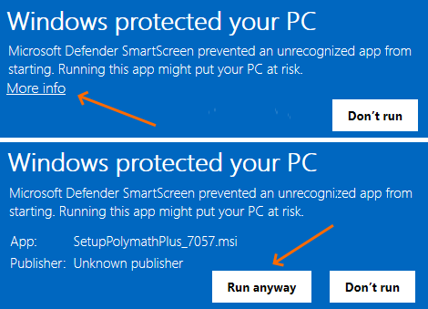
When you use Tools > Login in the desktop application, you may encounter the error: "Object reference not set to an instance of an object", and the application crashes.
This is a known bug in the older desktop release version SetupPolymathPlus_7051.msi.
To resolve this issue, please download and install the latest version from your profile page.
If you still wish to use an older version, please follow these steps to bypass the issue and complete the registration:
The Windows desktop application relies on the Microsoft Edge WebView2 Runtime. If Edge is not already installed on your computer, you will need to install the WebView2 Runtime separately.
If the application errors with 'The system cannot find the file specified (0x80070002)', download and install the WebView2 Runtime from the Microsoft link below:
 WebView2 Evergreen Bootstrapper
When solving nonlinear equations—whether a single equation or a system—write each equation so it equals 0 (root-finding form) and provide an initial guess for each variable. In other words, express each equation as 𝑓(𝑥)=0 and supply an initial guess for every nonlinear variable.
Here's a quick example showing how to set up and enter the data for solving two simultaneous nonlinear equations:
|
x2 + y = 12
2x + log(y+2) = 5 |
The unknown variables are x and y.
Below are the root expressions, each corresponding to one of the unknowns, along with initial estimates—both set to 1.
| • | Any part of a line starting with # is treated as a user comment. It's ignored during evaluation and has no effect on the calculations. |
| • | With implicit multiplication syntax, you may omit the multiplication operator * in some cases. For example, 2x is equivalent to 2*x. |
You can also define auxiliary expressions to help simplify long formulas. In the example below, we define a as an auxiliary expression—meaning it's treated as a separate, explicit variable that other expressions can reference. You don't need to provide initial guess for auxiliary explicit variables—they're automatically computed from the nonlinear variables with provided initial guess.
When solving a single nonlinear equation—even if you include as many explicit helper variables and expressions as you like—the way you set the starting values is a bit different. Rather than supplying only a single starting estimate, you are required to specify both a lower and an upper bound for the variable, shown as var(min) and var(max).
Take a look at this example where we solve a nonlinear equation to find the value of V.
When solving multiple linear equations, you can enter them in the standard format—just as you'd normally write them. There's no need to rearrange the equations or provide any initial guesses. Simply ensure that all the equations are truly linear.
Here's an example of three linear equations being solved simultaneously:
|
a + 2c = 50
b = −2 + c a + 23c = 12 + b |
The following equations should be entered into PolymathPlus to solve the system described above:
Using implicit multiplication simplifies the syntax:
Using an AI assistant?
Copy the PolymathPlus AI context.
PolymathPlus is designed to solve systems of simultaneous initial value problems (IVPs) involving first-order ordinary differential equations (ODEs).
Higher-order differential equations can be transformed into systems of first-order equations using standard mathematical techniques. Likewise, partial differential equations (PDEs) can be converted into ODEs for numerical solution using methods such as the method of lines.
Each equation in PolymathPlus must be written in first-order form, where the derivative of a dependent variable is isolated on the left-hand side and expressed as an algebraic function of independent and dependent variables. This structure ensures compatibility with the program's numerical solvers.
Consider this set of ordinary differential equations to be solved:
Given these initial and boundary conditions:
The equations can be entered in PolymathPlus using the following syntax:
You can also use either of the following two compatible syntax formats for the same problem:
The output shows a table of results along with an integration chart.
| Variable | Initial | Minimal | Maximal | Final Value |
| t | 0 | 0 | 1 | 1 |
| x | 1 | 1 | 4.465 | 4.4645367 |
| y | 4 | 3.736 | 4.22 | 3.7357297 |

In addition to differential equations, PolymathPlus allows users to define explicit variables—algebraic expressions that depend on differential variables, the independent variable, and/or other explicit variables, provided no circular dependencies exist. These variables are computed directly from known values and can be used to simplify equations, define intermediate results, or support the overall structure of the model.
The example below illustrates a typical input format for solving a system of ordinary differential equations (ODEs) in PolymathPlus, including the use of explicit helper variables.
Where the initial values of XG and v are 1, 0 respectively, and the boundary conditions of t are t0 = 0 and tf = 3.
The source code to solve this system of ordinary differential equations:
When using implicit multipliers and shorter syntax, we can simplify the program to:
Using an AI assistant?
Copy the PolymathPlus AI context.
PolymathPlus supports curve fitting for linear, polynomial, multi-linear, and nonlinear regression. The report evaluates model variables, generates a regression chart and residual plots, and provides statistics on model accuracy.
When analyzing tabular data for curve fitting, choosing the correct regression model is essential for accurate forecasting and parameter estimation. The following examples use the same six-point dataset to demonstrate how PolymathPlus handles different regression commands, and how to use the solver's statistical output to determine the best model fit.
When analyzing tabular data, the simplest approach is often a straight-line fit. By setting the polynomial order to 1, PolymathPlus performs a standard linear regression ().
The following example demonstrates how to use the polyfit command to perform a linear regression on the dataset enclosed by [ ]. The first row inside the dataset must be the variables names.
The linear regression solution results are shown in the tables below:
| Variable | Value | 95% confidence |
| a0 | -4.6405288 | 4.22502 |
| a1 | 5.4996764 | 1.07763 |
| R² | R²adj | Rmsd | Variance |
| 0.980461 | 0.975576 | 0.549421 | 2.71677 |

Statistical Interpretation:
While the linear model yields a seemingly high R2 of 0.98, analyzing the parameter confidence intervals reveals a problem. The solver estimates the intercept a0 as -4.64, but the 95% confidence interval is extremely large (4.22). An error margin this large relative to the parameter's value indicates that the straight-line model struggles to fit the underlying mechanics of the data, which clearly contains curvature.
To capture the curvature missed by the linear model, we increase the polynomial order to 2 to perform a quadratic regression (). PolymathPlus calculates the optimal coefficients, including a free y-intercept parameter.
The polynomial regression solution results are shown in the tables below:
| Variable | Value | 95% confidence |
| a0 | 0.014488281 | 0.706117 |
| a1 | 1.9324766 | 0.463760 |
| a2 | 0.51325831 | 0.0652076 |
| R² | R²adj | Rmsd | Variance |
| 0.999907 | 0.999845 | 0.0379046 | 0.0172411 |
Statistical Interpretation:
This model drastically improves the fit, achieving an R2 of 0.9998. However, looking closely at the parameters, the solver estimates the intercept a0 as 0.014, but its 95% confidence interval is 0.706. Because the confidence interval is larger than the parameter value itself, the intercept is statistically indistinguishable from zero. This tells us the model is over-parameterized and a0 should likely be dropped.
In many engineering problems, the model must pass exactly through zero. By appending the origin keyword to the command, PolymathPlus forces the y-intercept to zero, optimizing only the x and x2 coefficients.
The polynomial regression via the origin solution results are shown in the tables below:
| Variable | Value | 95% confidence |
| a0 | 1.9412543 | 0.135379 |
| a1 | 0.51213773 | 0.0269368 |
| R² | R²adj | Rmsd | Variance |
| 0.999907 | 0.999884 | 0.0379315 | 0.0129492 |

Statistical Interpretation:
This is the strongest model. It maintains an excellent R2 (0.9999), and because we removed the unnecessary free intercept, the remaining parameters now show exceptional precision. The solver returns a0 (the x term) as 1.941 ± 0.135 and a1 (the x2 term) as 0.512 ± 0.0269. With tight 95% confidence bounds and high variance explained, this model fits the data very well.
Polynomial regression is a special case of multiple linear regression in which nonlinear terms—such as x2—are computed beforehand and included as additional predictor variables. You can pre-calculate these transformed features and place them directly in your data table.
In this example, the x2 values appear as a separate column named x2. This approach is especially useful when working with raw datasets that already contain derived or interaction features.
Note: mlinfit requires listing all predictor variables first, followed by the dependent variable last.
The Multilinear regression model solution becomes:
| Variable | Value | 95% confidence |
| a0 | 0.014488281 | 0.706117 |
| a1 | 1.9324766 | 0.463760 |
| a2 | 0.51325831 | 0.0652076 |
| R² | R²adj | Rmsd | Variance |
| 0.999907 | 0.999845 | 0.0379046 | 0.0172411 |
Statistical Interpretation:
The solver treats x and x2 as independent predictor columns. Because the underlying data matrix is identical, the resulting R2 and parameter confidence intervals will match the polynomial fit polyfit x y 2 exactly.
PolymathPlus allows you to explicitly define mathematical transformations as helper variables outside the data table, and then feed them into the mlinfit command (same applies to the polyfit and nlinfit commands).
In this example, we define an explicit variable x2 as x2 and pass both predictors to the solver.
The solver output for this model yields the exact same statistical results (R2 and confidence intervals) as the standard second-order polynomial fit polyfit x y 2, as well as the multilinear regression example above.
Just like the polyfit command, mlinfit also supports the origin keyword. By adding origin to the end of our transformed multilinear regression, we force the intercept of the multilinear plane to zero.
The multiple linear regression via the origin solution becomes:
| Variable | Value | 95% confidence |
| a0 | 1.9412543 | 0.135379 |
| a1 | 0.51213773 | 0.0269368 |
| R² | R²adj | Rmsd | Variance |
| 0.999907 | 0.999884 | 0.0379315 | 0.0129492 |

Statistical Interpretation:
Because our predictors are x and x2, this formulation is mathematically identical to the second-order polynomial regression via the origin. The solver returns the exact same parameter results and tight confidence intervals.
Below is an example of a data entry for solving nonlinear regression model for a given set of data points. The model variables to be found are a and b, for which we should also provide an initial guess.
The model eqaution to fit is as follows:
The data entry for this nonlinear regression model is as follows:
The nonlinear regression solution becomes:
| Variable | Initial guess | Value | 95% conf. |
| a | 2 | 1.32753 | 0.0269902 |
| b | 1 | 0.0264615 | 0.00285336 |
| R² | R²adj | Rmsd | Variance |
| 0.998802 | 0.998502 | 0.00440595 | 0.000174712 |

PolymathPlus can calculate a definite integral from known discrete data points. The solver interpolates the supplied data, builds a continuous curve and calculates the area under the curve over the requested interval. This is useful when the function is known through measurements or simulation output tabulated data rather than through a closed-form equation.
In this example, PolymathPlus integrates y(x) from x = 3 to x = 8.6. The tabulated values of x are given explicitly in the data table, and the tabulated values of y are calculated from the values of t.
The solution report shows the integral calculated from the data points and a chart with the interpolated curve and the area from which the integration is derived.

Internally the default algorithm implements the Akima interpolation with Simpson integration using 100 sub-sections. Optional command arguments to the integrate command provide direct control when needed: use integrate y(x) 2 3 90 akm for Akima interpolation over 2-3 with 90 sub-sections, integrate y(x) 1 2 50 ccs for CCS interpolation over 1-2 with 50 sub-sections, or integrate y(x) 5 9 80 lin for linear interpolation over 5-9 with 80 sub-sections.
The default settings are designed to work well in almost all practical cases. Advanced users can still override the defaults by choosing the interpolation method and the number of sub-sections used for the numerical integration. Increasing the number of sub-sections can improve accuracy for rapidly changing curves.
Using an AI assistant?
Copy the PolymathPlus AI context.
PolymathPlus solves constrained nonlinear programming (NLP) problems. It minimizes a nonlinear objective function by adjusting model variables within user-defined bounds and constraints. Once the lowest feasible objective value is found, the software generates summary reports, charts, and statistics to evaluate the quality of the model fit.
To set up an NLP problem, start by specifying the objective function you want to minimize using the min: keyword.
Constraints are added as expressions that must equal zero for equality constraints (use ... = 0),
or be greater than zero for inequality constraints (use ... > 0).
Write each constraint as a mathematical expression followed by the appropriate comparison.
Please Note: Be sure to rewrite each constraint so that all terms appear on one side of the equation or inequality, leaving zero on the other side.
A key requirement for the NLP solver is to provide bounds for each variable.
For every variable, you must enter an initial guess, a lower bound, and an upper bound
in the following format: variable | guess lower_bound upper_bound
This helps the solver search only within the meaningful range for your model.
The following example demonstrates how to set up a constrained optimization problem. Here, the objective is to minimize a squared distance function subject to nonlinear inequality constraints that define the feasible region.
Mathematically, the problem is formulated as:
The corresponding data entry and the solution report are as follows:
the solution report shows the optimal values of the variables, the final minimized value of the objective function, and statistics on the quality of the fit.
| Variable | Initial | Lower | Upper | Optimal |
| x | 1.6 | 0 | 10 | 2.0000112 |
| y | 1.3 | 0 | 10 | 3.0000474 |
| Var | Score | Grad | StdErr | RelStdErr |
| x | 5 / 10 | 2.23E-5 | 0.707 | 35.4% |
| y | 4 / 10 | 9.478E-5 | 0.707 | 23.6% |
Convergence Analysis
Progress per iteration

Since the global minimum of the function is located at and this point satisfies all constraints (where and ), the solver converges to the optimal value of .
Least Squares (LSQ) optimization is a specific type of nonlinear programming (NLP) used to fit mathematical models to observed data. The main goal is to minimize the sum of squared differences (residuals) between the actual data points and the values predicted by the model. This approach is widely used in scientific modeling, as it provides a quantitative measure of how well the model matches the data under various equality and inequality constraints.
To perform LSQ optimization in PolymathPlus, you provide a set of observed data points and define a mathematical model that describes the relationship between variables. The solver then adjusts the model parameters to find the best fit, minimizing the total squared error.
Below is an example of how to enter data for a least squares optimization problem. In this example, the model uses a saturation kinetics form (which is commonly applied in enzyme kinetics and other scientific fields). The objective is to find the parameter values that make the model curve fit the data points as closely as possible.
The saturation kinetics form model:
The equation above represents a common model used to describe how a response variable y changes with respect to an independent variable x, where - we seek to find the best fitting model variables Vmax (represented by a) and Km (represented by b), by minimizing the residuals of calculated ycalc values compared to the observed y data points.
In the PolymathPlus program, we should define the data-table of the known variable. We should also define the model expression to optimize using the fit: keyword followed by the math expression. In this case, we write fit: y = a*x/(b + x)
The program will attempt to find the best suited model variables a and b, by minimizing the sum of squared residuals:
Here is the PolymathPlus program to solve the LSQ optimization problem described above:
This is the solution result of the optimization process:
| Variable | Ini | Lower | Upper | Optimal |
| a | 1.5 | 0 | 5 | 2.0000307 |
| b | 0.3 | 0 | 5 | 0.50004194 |
| R² | R²adj | SSE | RMSE | σ² | DOF |
| 1 | 1 | 1.2e-9 | 1.5e-5 | 3.2e-10 | 4 |
| Variable | StdErr | 95% Confidence |
| a | 3.36e-4 | 1.85e-4 |
| b | 2.22e-4 | 1.28e-4 |
The verified solution for this dataset yields a ≈ 2.0 (representing Vmax) and b ≈ 0.5 (representing Km). By evaluating the residual plots provided in the report, users can confirm that the error is randomly distributed, indicating that the nonlinear model chosen is an appropriate fit for the data.
The program solution report includes charts to visualize the accuracy of the fit:

Using an AI assistant?
Copy the PolymathPlus AI context.
PolymathPlus began as a Windows desktop application and expanded its offerings to include an online web application. Our passion and dedication drive us to continually innovate and refine our solutions. We are committed to providing a top-notch numerical solver package to tackle mathematical challenges with ease and confidence.
 |
admin@polymathplus.org
sales@polymathplus.org |
 |
Email us to schedule a call |
| Pre-scheduled calls only 08:00-10:00 AM ET |
|
 |
Maintenance Status |
The development of our software had been encouraged by CACHE - The Computer Aids for Chemical Engineering Education Corporation, as part of the American Institute of Chemical Engineers.
Drawing from more than 25 years of software development and extensive research in numerical packages, we have crafted the new PolymathPlus package. We maintain ties with many US-based universities and colleges, as well as institutions across other regions worldwide.
Deliver the premier user-friendly, advanced math solver—accessible and affordable worldwide—the first choice for learners, professionals, and enthusiasts.
Our research is dedicated to advancing numerical methods and optimization techniques to strengthen the capabilities of PolymathPlus. The following key research areas highlight their potential impact across disciplines commonly applied in science and engineering, particularly in design, modeling, and control.
The Simplex method solves linear programming problems by moving along the edges of feasible solutions to find the optimal one. Enhancing Simplex algorithms with advanced pivot rules, degeneracy handling, and dual simplex implementations to handle large-scale linear optimization problems more efficiently. Research includes interior-point methods and revised simplex algorithms for improved numerical stability.
Optimization solvers locate a function’s minimum or maximum, with support for constraints and variable bounds. Engineers use methods such as Gradient Descent, Conjugate Gradient, BFGS, and L‑BFGS to improve convergence and reduce computation time. Constrained problems are handled with techniques like Augmented Lagrangian, GRG, and KKT conditions, which ensure feasible and efficient solutions in complex systems.
Chebyshev and Fourier transformations are mathematical tools used to represent functions using orthogonal basis sets. They enhance numerical solvers for discrete data, improving accuracy and computational efficiency in interpolation and approximation. These transformations also enable advanced solvers by replacing discrete data with continuous function representations.
We investigate hybrid numerical workflows that combine nonlinear equation solvers, optimization methods, and ODE solvers. These integrated approaches support boundary‑value ODE problems and ODE‑based curve fitting, where parameters are optimized to match dynamic system behavior. The goal is to build flexible algorithms that unify simulation, parameter estimation, and numerical solving.
Solving partial differential equations is central to modeling physical phenomena in engineering and science — from heat transfer and fluid dynamics to structural mechanics, convection–diffusion–reaction systems, and electromagnetics. Common approaches for numerical solvers include the relatively simple yet constrained method of lines (MOL), finite difference methods for structured grids, finite element methods for complex geometries, and spectral methods for high‑precision solutions.
These research efforts represent our ongoing commitment to improving computational mathematics. While we work to incorporate these advancements into PolymathPlus, we aim to provide users with reliable and efficient tools for solving complex mathematical problems.
Below are sample reports generated by solving PolymathPlus programs. The input for each program is shown at the top of every report. Each group features example problems and their corresponding solution reports.
Start solving as a guest, then register for free to unlock more features.
Using an AI assistant?
Copy the PolymathPlus AI context.
Terms and Conditions PolymathPlus does not warrant that the functions contained in the program will meet your requirements or that the operation of the program will be uninterrupted or error-free. In no event will PolymathPlus or its distributors or their dealers be liable to you for any damages, including any lost profit, lost savings, or other incidental or consequential damage. Please read the Terms of Service (TOS) below for further details.
